All firms (ONS, 2023–24)
VAT-registered firms (HMRC, 2023–24)
An open firm-level model for UK VAT threshold reform
Abstract.
I present an open, reproducible firm-level microsimulation for costing UK VAT registration-threshold reforms, released with its synthetic-data generator. The threshold is a notch: once turnover crosses £85,000, 20% VAT falls due on a firm’s whole turnover, not the excess. I build synthetic firm records from ONS counts, calibrate them to 2023–24 HMRC statistics, and cost level, shape (a taper) and rate (a reduced-rate band) reforms statically on a common basis, reproducing HMRC’s £85,000-to-£90,000 costing within £10m. I characterise the notch by its dominated region—the exact £21,250 band above the threshold in which no firm locates—and how each reform changes it: raising it (to £100,000, \(-\)£508m) relocates it, a reduced rate shrinks it, a taper removes it. I price level and rate reforms behaviourally, conditional on an assumed elasticity, as a sensitivity range nesting the static cost. A placebo shows the synthetic bunching is a calibration artefact, not behaviour.
Keywords: value-added tax, microsimulation, tax notch, policy
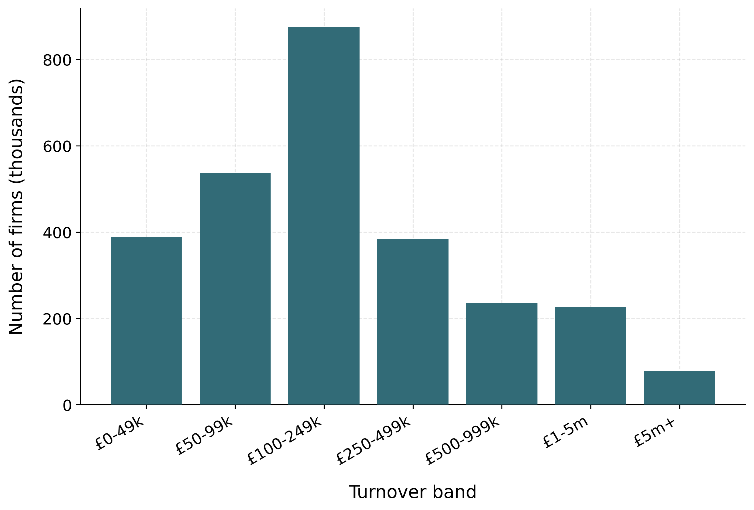
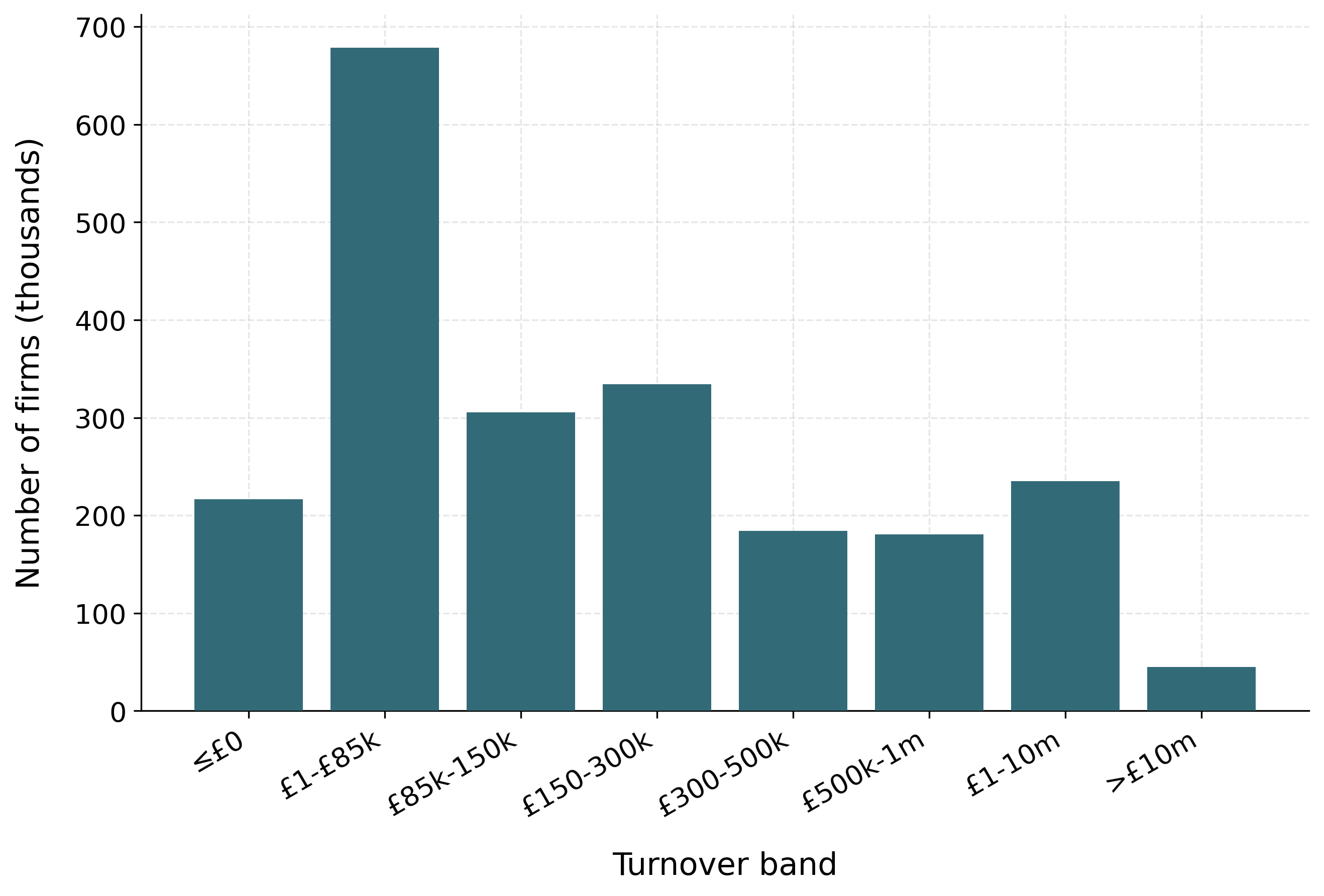
The United Kingdom’s Value Added Tax (VAT) applies above a registration threshold that is among the highest in the OECD (Seely 2024; HM Revenue and Customs 2024). The threshold is a notch rather than a kink: once a firm’s annual taxable turnover crosses it, the standard 20% rate falls due on all of the firm’s turnover, not only on the part above the threshold, so registration produces a discrete jump in liability rather than a marginal one. The threshold falls in a dense part of the firm distribution. Figure 1(a) shows that UK firms are concentrated at the lower end of the turnover distribution, and Figure 1(b) shows that VAT-registered firms are concentrated in the turnover bands at and below the threshold, so the notch applies to a large number of firms.
All firms (ONS, 2023–24)
VAT-registered firms (HMRC, 2023–24)
Firms respond to the notch by locating below the threshold. Tabulations of HMRC turnover data show the number of firms rising towards £84,000 and then dropping sharply at the £85,000 threshold, leaving excess mass just below it (Office for Budget Responsibility 2023). Liu et al. (2021) document this bunching in UK firm data, and Liu et al. (2024) find that firms slow their turnover growth as they approach the threshold. The notch therefore distorts the size distribution and the growth decisions of firms near the margin, which places the threshold under recurrent pressure for reform.
Reform proposals change the threshold in one of three ways: its level (raising or lowering it), its shape (replacing the notch with a schedule that phases the rate in over a band), or its rate (a reduced rate for firms in a band above the threshold). The three are not equivalent. Changing the level moves the notch along the turnover axis; changing the shape or the rate alters the size of the discrete jump itself. Costing the three on a common basis is the practical difficulty this paper addresses. A change in the level can be costed by mechanical accounting, but a change in the shape of the schedule cannot be evaluated with the reduced-form bunching methods used to study the threshold, because a continuous schedule leaves no single point of excess mass to exploit. The firm-level data needed to study turnover near the threshold is, in addition, not available in open form.
In this paper I build an open, reproducible firm-level microsimulation for costing UK VAT threshold reforms on a common static basis. I construct synthetic firm microdata calibrated to published HMRC aggregates—band-level firm counts and sector turnover totals—for the 2023–24 tax year, when the threshold was £85,000 (raised to £90,000 in April 2024); the synthetic data can be released openly and regenerated under any counterfactual schedule. On these data I do four things. I cost both level reforms and schedule reforms—a graduated taper and a reduced-rate band—statically, by applying each counterfactual schedule mechanically to the firm distribution. I show that the synthetic data reproduce the density step at the £85,000 notch documented in administrative data by Liu et al. (2021), and I use a placebo test to demonstrate that this step is mechanical—inherited from the coarse band-level counts that serve as calibration targets rather than generated by firm location choice—so I draw no behavioural elasticity from the synthetic bunching. And I characterise the notch’s distortion through its dominated region—the exact, model-free range of turnover above the threshold in which no firm locates—and how each reform changes it. I then additionally price the reforms behaviourally: a structural simulator re-optimises each firm under each counterfactual schedule—a forward solve that re-prices firms rather than applying the schedule to the observed distribution—conditional on an assumed turnover elasticity \(e\) that I do not identify from the data, and I report the result as an \(e\)-sensitivity range that nests the static costing in its \(e\to0\) limit. The static cost and the exact dominated region remain the elasticity-free robust anchors.
Three findings follow. First, the static pipeline prices level and shape reforms on a common basis and reproduces HMRC’s published anchor costing: my static costing of the April 2024 increase from £85,000 to £90,000 gives £175m in 2025–26 against HMRC’s published £185m, agreeing within about £10m—an internal-consistency check on the costing rather than an external validation. Forward moves from the £90,000 base range from a gain of £665m at £70,000 to a cost of £1,205m at £120,000, against a base of about £203.8bn.
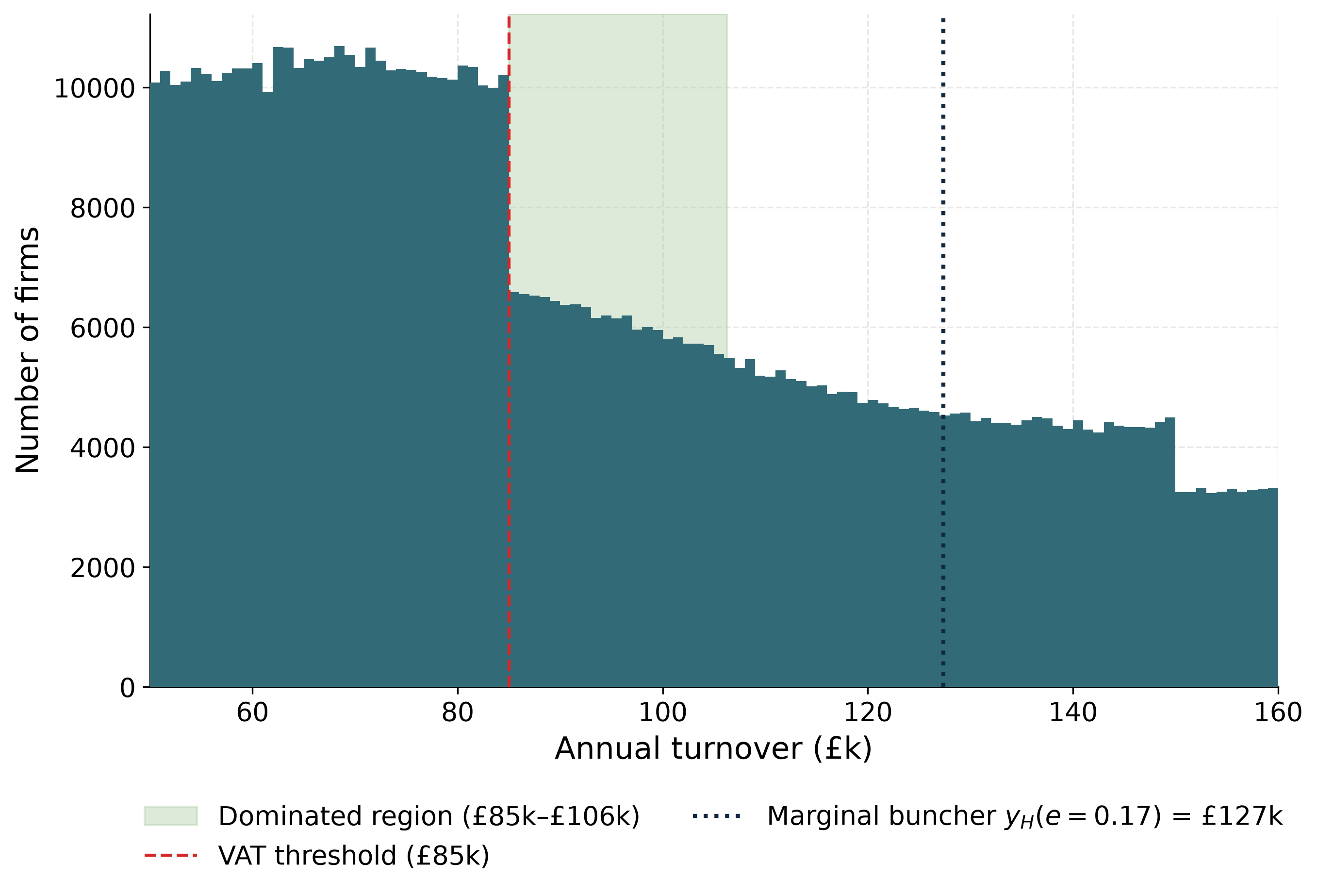
Second, the shape and rate reforms act on the notch’s distortion in a way that a change in level does not. The notch creates a dominated region of width \(a = T^{*}\tau/(1-\tau) = \pounds 21{,}250\) above the threshold (£85,000–£106,250), a range of turnover in which no firm can locate without being strictly worse off than at the threshold. This region is an exact, model-free property of the schedule: it follows from the arithmetic of the notch alone and requires no behavioural calibration. It also spans a populous part of the firm distribution—about 137,000 weighted firms—so its width is an economically meaningful distortion index, not a theoretical curiosity. Raising the threshold relocates this region without removing it. A reduced rate shrinks it—to £9,444 at a 10% band rate and £15,000 at 15%—while a graduated taper, being continuous, removes it. Set against their static revenue costs, the reforms are not interchangeable: raising the threshold to £100,000 costs £508m, the most expensive option, yet removes none of the distortion; the taper removes the dominated region entirely for £336m; and the 10% and 15% reduced rates cost £343m and £171m while shrinking it. The level move is therefore the dearest and least efficient of the menu. I report, for each reform, its static cost together with the portion of the dominated region it removes.
sticity-free anchors.
Third, the open data carry a transparency lesson about bunching. The synthetic records reproduce the density step at £85,000 that Liu et al. (2021) document in administrative data, which might tempt one to read a behavioural response off the synthetic distribution. A placebo test shows this would be a mistake: when the density step is removed from the calibration target, the apparent excess mass collapses from about 8,712 firms to roughly 99, revealing that the step is mechanical—a reflection of the two coarse turnover bands HMRC publishes across the threshold, baked into the calibration target—rather than a product of firm location choice, which the generator does not model. Behavioural bunching is thus not identified on the synthetic data, and I make no such claim from them; the behavioural evidence remains Liu et al. (2021)’s administrative estimate. I treat the reproduction of the published step as a credibility check on the data and the placebo as the appropriate caveat against over-reading it.
Related literature. The paper draws on and contributes to four strands of work. The first is the methodology of bunching and notches (Saez 2010; Kleven and Waseem 2013; Chetty et al. 2011; Kleven 2016; Best et al. 2015), which provides the analytic notion of a dominated region; I use the dominated region to characterise a distortion that leaves no single point of excess mass to exploit. The second is the empirical literature on the VAT registration threshold (Liu et al. 2021, 2024; Onji 2009; Harju et al. 2019; Asatryan and Peichl 2017; Nandi and Warwick 2020; Bashir et al. 2024), which estimates the behavioural response and studies changes in the threshold’s level. Liu et al. (2021) is closest: it estimates bunching at the UK notch on administrative data and documents voluntary registration; I take its administrative estimate as the established behavioural fact, show that my open synthetic data reproduce the density step it documents, and cost shape and rate reforms statically on a common basis. The international evidence (Harju et al. 2019; Onji 2009; Asatryan and Peichl 2017; Nandi and Warwick 2020) notes that bunching at a VAT threshold can reflect compliance costs, firm-splitting, or reporting rather than real turnover responses. The third strand questions whether bunching identifies a structural elasticity at all: Blomquist et al. (2021) show that the elasticity is not non-parametrically identified from bunching at a kink without strong functional-form assumptions, and Bertanha et al. (2023) make the analogous point for notches. This literature motivates my refusal to read a behavioural elasticity off the synthetic bunching: even setting aside the placebo evidence that the synthetic step is mechanical, the mapping from excess mass to an elasticity is not identified without assumptions I am unwilling to impose. The fourth strand is the structural literature on size-based thresholds (Garicano et al. 2016; Gourio and Roys 2014), which identifies policy-invariant primitives at the French 50-employee threshold and computes welfare from them; the present paper makes no such structural claim, pricing reforms statically and, conditional on an assumed elasticity, behaviourally. This paper makes three contributions. First, it provides an open, reproducible firm-level microsimulation for costing UK VAT threshold reforms, where the existing firm-level evidence on the threshold rests on restricted administrative data; as part of this, I show transparently that the open data reproduce the published density step and use a placebo to establish that the step is mechanical, so no behavioural bunching is claimed from the synthetic data. Second, it characterises the notch’s distortion through its exact, model-free dominated region and costs two schedule reforms—a graduated taper and a reduced-rate band—on the same static basis as level reforms, where prior work has neither costed these reforms nor measured this distortion. Third, it prices these reforms behaviourally with a structural simulator that re-optimises each firm under each schedule, conditional on an assumed turnover elasticity, reported as a sensitivity range that nests the static costing in its zero-elasticity limit. Because the synthetic data do not identify the turnover elasticity, identifying it from administrative micro-data is what remains for future work; a welfare and marginal-value-of-public-funds accounting—together with revenue-neutral designs and the treatment of voluntary registration—are also left for later.
The remainder of the paper proceeds as follows. Section 2 describes the institutional background of the UK VAT threshold. Section 3 sets out the synthetic firm microdata and its calibration to HMRC aggregates. Section 4 sets out the static costing of threshold changes and the schedule reforms. Section 5 reports the reduced-form bunching evidence. Section 6 develops the notch and its exact dominated region, and shows how each reform changes it. Section 7 prices the reforms behaviourally with a structural simulator conditional on an assumed elasticity, reported as a sensitivity range that nests the static costing. Section 8 concludes.
The United Kingdom levies a value-added tax at a standard rate of 20% on most goods and services. A business must register once its taxable turnover over any rolling twelve-month period exceeds the registration threshold, after which it charges VAT on its taxable sales and reclaims VAT paid on inputs. Because registration makes VAT due on the firm’s entire taxable turnover rather than only the amount above the cutoff, the threshold is a notch—a discrete jump in liability—and not a kink. The cost of crossing is largest for consumer-facing firms with limited pass-through and small reclaimable input shares, for whom the incentive is to restrain turnover and locate just below the threshold (Liu et al. 2021; Kleven and Waseem 2013).
Real VAT is a tax on value added, not on turnover: a registered firm charges output VAT on its sales but reclaims input VAT on its purchases. A large share of below-threshold firms therefore register voluntarily—roughly \(43\%\) of eligible below-threshold firms (Liu et al. 2021), driven by input-VAT reclaim and business-to-business sales—and for them the incentive to bunch is weak. My one-input model taxes turnover rather than value added, so it is a turnover-tax-notch approximation for the consumer-facing, limited-reclaim firms for whom the bunching incentive is sharpest; it abstracts from input reclaim and voluntary registration. I treat this as a first-order scope restriction.
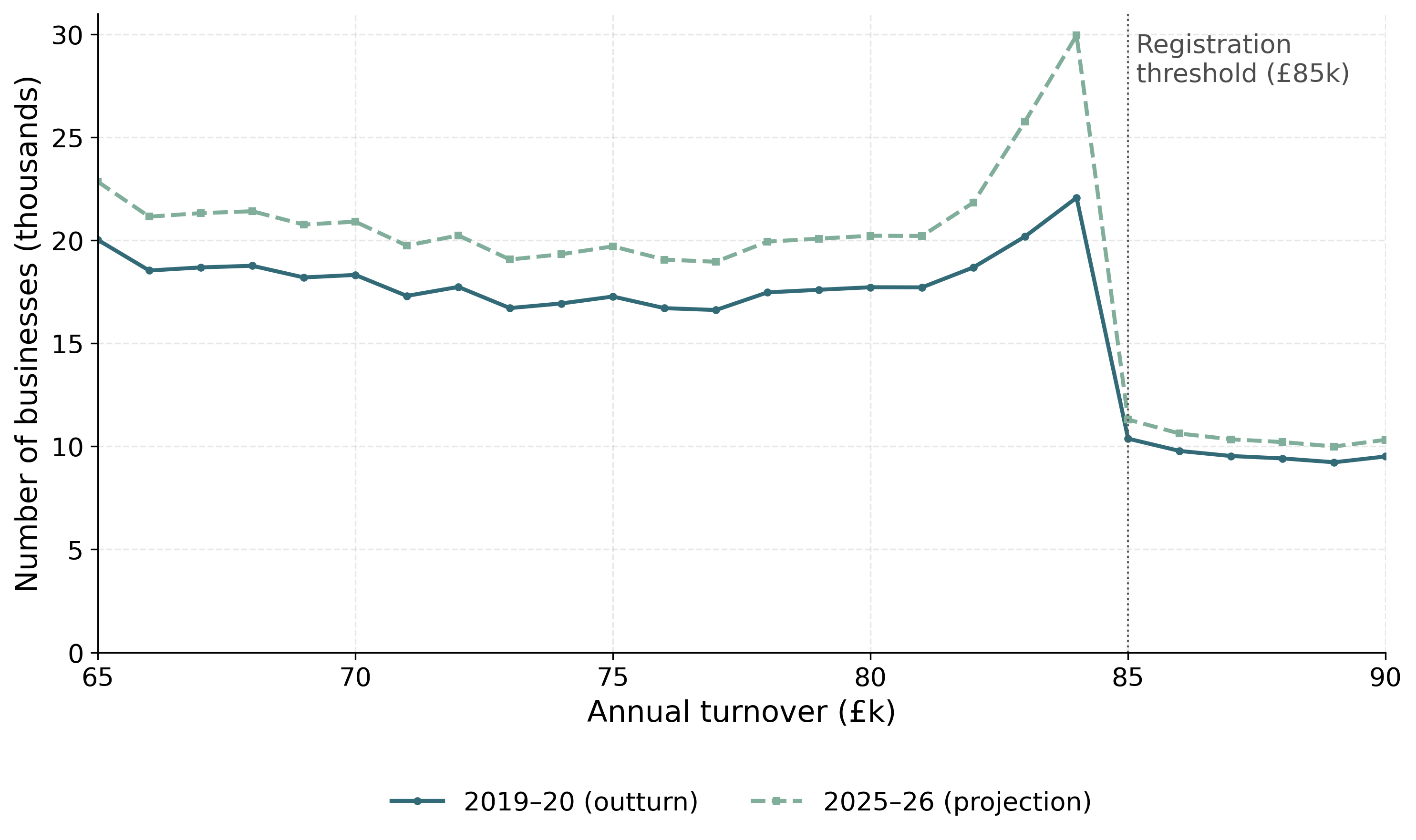
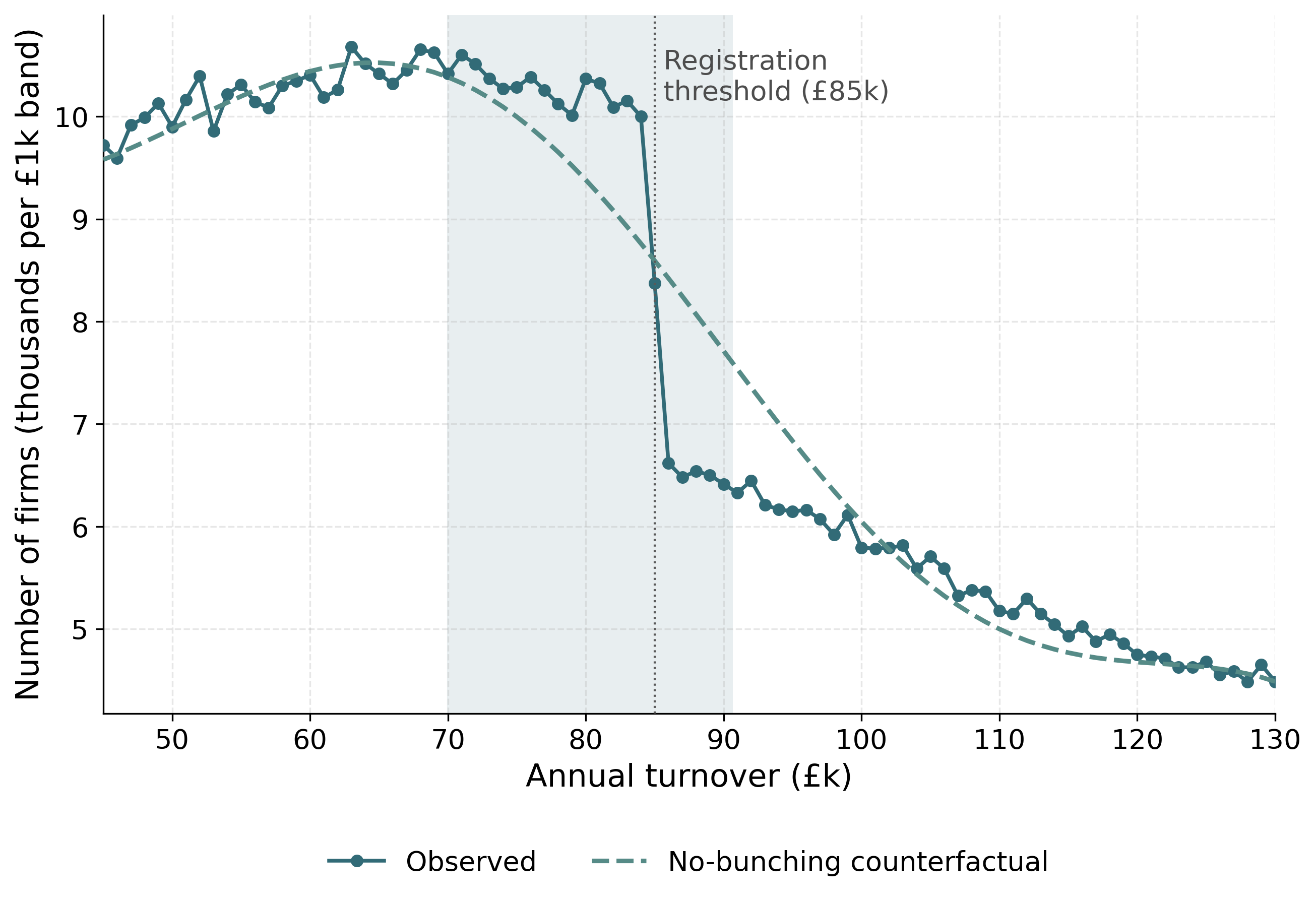
The registration threshold was held at £85,000 from 1 April 2017 to 31 March 2024—a seven-year nominal freeze, the longest in the history of the tax—before being raised to £90,000 on 1 April 2024, with the deregistration threshold rising from £83,000 to £88,000 (HM Revenue and Customs 2024; Seely 2024). Because nominal turnover grows with inflation and real activity, freezing the threshold lowers it in real terms and draws an increasing number of firms towards the registration margin; this fiscal-drag mechanism was a central motivation for the April 2024 increase. My data year is 2023–24, so the prevailing statutory threshold throughout my analysis is £85,000. Figure 2 shows the pattern in the turnover distribution: the number of firms rises towards £84,000 and falls sharply above £85,000, and the projected 2025–26 distribution is more sharply bunched than the 2019–20 outturn as fiscal drag draws more firms towards the frozen threshold.
The UK threshold is among the highest in the OECD, and there is debate over whether to raise it—to reduce the compliance burden on small firms—or lower it, to broaden the base and reduce the growth distortion at the margin. Three families of reform feature, and I evaluate all three: a change in the threshold’s level (the £85,000 to £90,000 increase of April 2024 and further moves around it); a change in its shape (a graduated taper that phases the effective rate in over a band, replacing the notch with a continuous profile); and a change in its rate (a reduced rate for small firms in a band above the threshold, with the standard 20% rate retained above). The taper and reduced-rate designs follow proposals in the UK policy debate, notably Office of Tax Simplification (2017), which canvassed a financial incentive or reduced effective rate to smooth the cliff-edge at the threshold. A banded reduced rate introduces a smaller secondary notch at the band top, which the continuous taper avoids. I cost all three by the same machinery in Section 4.
Studying firm responses at the threshold needs firm-level turnover near the cutoff, which the official statistics publish only in coarse turnover bands. I therefore build a synthetic firm population calibrated to those aggregates: it reproduces the official totals while resolving the individual firm that the authorities do not release, opening the analysis to anyone. The same calibrate-to-published-aggregates approach underlies open household-level tax-benefit microsimulation (PolicyEngine 2025); here I apply it at the firm level. The generator takes the registration threshold as a parameter and is documented in Appendix 9.1.
Index firms by \(i\). For each sector \(s\) and ONS turnover band \(b=[\underline{b},\overline{b}]\), the UK Business: Activity, Size and Location table gives a firm count \(N_{s,b}\), and I draw \(N_{s,b}\) firms with within-band turnover \[y_i \;=\; \underline{b} + (\overline{b}-\underline{b})\,u_i + \varepsilon_i, \qquad u_i \sim \mathcal{U}(0,1), \;\; \varepsilon_i \sim \mathcal{N}(0,\sigma_b^2),\] truncated below at zero, where \(\varepsilon_i\) smooths the within-band distribution. Each firm is given input expenditure \(x_i = \rho_i\,y_i\), with the input–output ratio \(\rho_i\) drawn from a rescaled Beta distribution with sector-specific shifts and bounded to \(\rho_i \in [0.6,1.5]\); its value added, the net VAT base, is \(v_i = y_i - x_i\). Employment is assigned from the ONS employment-band shares.
The base population reproduces the ONS structure but not the HMRC VAT-registered totals, so I re-weight it. Each firm receives a strictly positive weight \(w_i = e^{\theta_i}\), and for a vector of official targets \(T=(T_k)_{k=1}^{K}\) the weighted synthetic counterpart of target \(k\) is \[\widehat{T}_k(\theta) \;=\; \sum_i a_{ki}\, w_i ,\] where \(a_{ki}\) is firm \(i\)’s contribution to target \(k\): an indicator of band or sector membership for a count target, and the firm’s liability \(v_i\) for a VAT-liability target. I choose \(\theta\) to minimise a symmetric relative-error loss with per-target importance weights \(\lambda_k\), \[L(\theta) \;=\; \frac{1}{K}\sum_{k} \lambda_k \min\!\Big\{ \big(\widehat{T}_k/T_k - 1\big)^2,\; \big(T_k/\widehat{T}_k - 1\big)^2 \Big\} \;+\; \frac{\alpha}{N}\sum_i \lvert \theta_i \rvert ,\] the final term a mean absolute penalty on the log-weights. The targets are the HMRC VAT-registered counts by turnover band and by sector, the HMRC net VAT liability by turnover band, and the ONS employment-band totals; turnover-band targets carry the largest \(\lambda_k\), followed by VAT liability by band. VAT liability by sector is reported as an informational diagnostic but excluded from the optimizer, because the current generator fixes firm inputs rather than calibrating the input/output tax structure by sector. The problem is solved by gradient descent, and the symmetric loss keeps targets of very different magnitudes on a common scale.
A firm is registered with certainty when its turnover exceeds the threshold \(T^{*}\). Below the threshold it registers voluntarily with probability \(r = M / n_{<}\), where \(M\) is the HMRC count of registered firms in the £1–threshold band and \(n_{<}\) is the unweighted number of synthetic below-threshold firm rows. This sets the expected row-level voluntary-registration rate; I do not treat below-threshold voluntary registration as a separate weighted calibration target. The resulting dataset comprises approximately \(2.94\) million firm records, weighted to represent roughly \(2.5\) million UK firms; checked for consistency against the official sources along every calibrated dimension, it attains an overall calibration accuracy of about \(90\%\). This headline is the mean of five calibrated-dimension scores, each clipped at zero as \(\max\{0,1-\lvert \widehat{T}-T\rvert/\lvert T\rvert\}\); it excludes the VAT-liability-by-sector diagnostic described above.
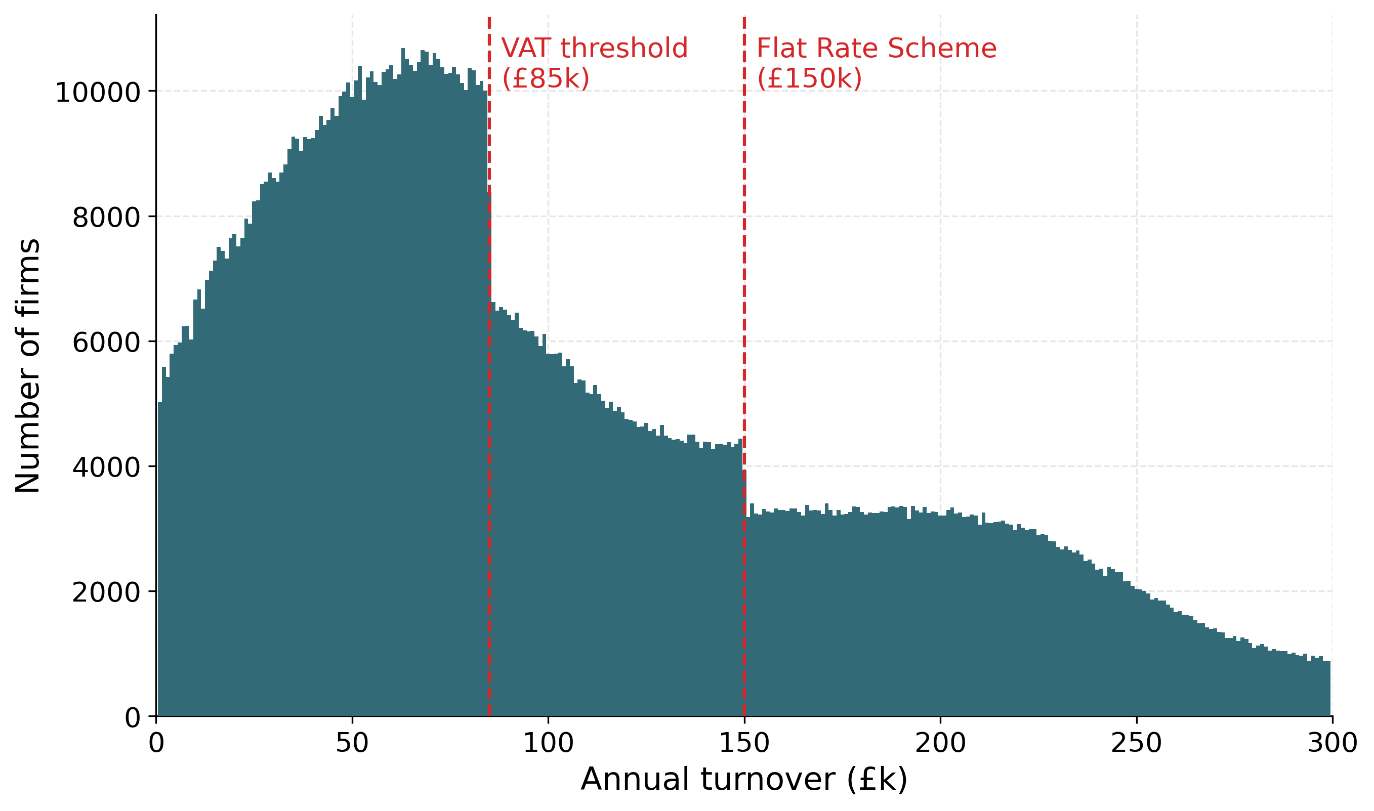
My data are for the 2023–24 year, in which the statutory threshold was £85,000. The firm density steps down at the threshold—from roughly \(10{,}200\) to \(6{,}600\) firms per £1,000 turnover band—reflecting the incentive to remain below the registration cutoff, with a second, smaller step at £150,000, the ceiling of the VAT Flat Rate Scheme (Figure 3). I note, however, that HMRC publishes firm counts only in coarse turnover bands across the threshold, so the density step at £85,000 in the synthetic data is inherited from these aggregate targets rather than from any modelled firm behaviour; Section 5 quantifies this with a placebo test. Counterfactual policies—including the £85,000 to £90,000 reform and the forward threshold sweep of Section 4—are evaluated on these firms by re-applying the registration rule to the microdata for the static costings. I hold the empirical turnover distribution fixed throughout. A fully behavioural forward solve that re-prices firms under counterfactual schedules is left to future work.
A static costing measures the first-order revenue effect of a reform by re-applying the tax rule to a fixed firm population, with no behavioural response. Let firm \(i\) have turnover \(y_i\), calibrated net VAT liability \(v_i\) (output less input VAT; Section 3), and weight \(w_i\). A firm remits VAT only once registered, that is once its turnover exceeds the threshold \(T\), so total VAT revenue at threshold \(T\) is the weighted sum of liabilities over registered firms, \[R(T) \;=\; \sum_i w_i\, v_i \,\mathbf{1}\{y_i \ge T\}.\] Because turnover is held fixed, moving the threshold from \(T_0\) to \(T\) changes revenue only through the firms whose registration status flips—those with turnover in the band between the two thresholds: \[\Delta R \;=\; R(T) - R(T_0) \;=\; -\,\operatorname{sign}(T - T_0) \sum_i w_i\, v_i \,\mathbf{1}\{\,T_{\min} \le y_i < T_{\max}\,\},\] where \(T_{\min}=\min(T,T_0)\) and \(T_{\max}=\max(T,T_0)\): lowering the threshold draws firms into the net and raises revenue, while raising it releases firms and loses revenue. The estimate is therefore the mechanical reclassification effect and excludes the behavioural response of Section 5. The calibrated weights reproduce HMRC’s net VAT-liability totals (Section 3), and I age the microdata to a given fiscal year by a cumulative nominal-growth factor. At the £90,000 threshold this puts total VAT revenue at £203.8bn in 2025–26 and £210.0bn in 2026–27.
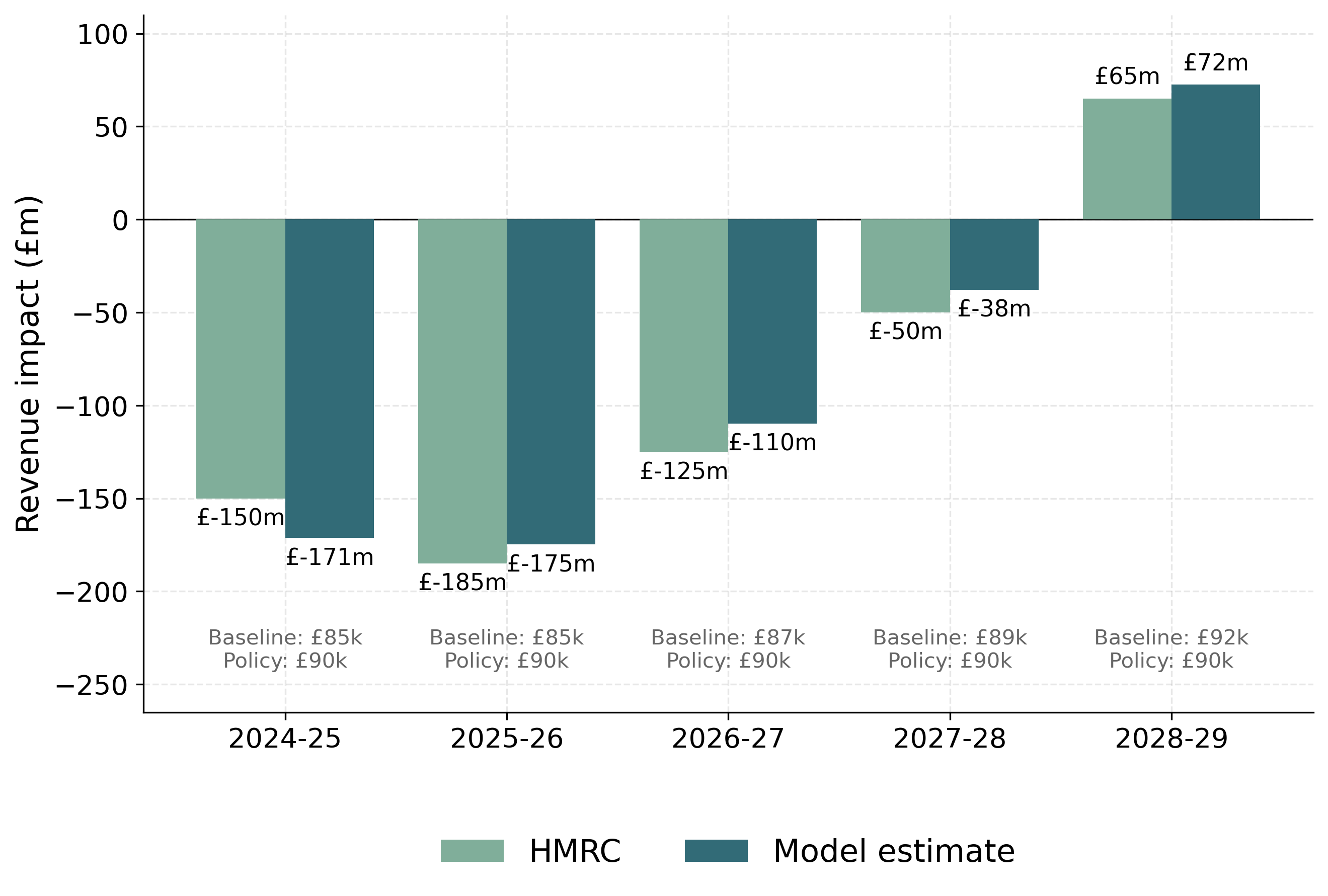
I first check the static pipeline against HMRC’s own costing of the April 2024 increase from £85,000 to £90,000. Because my microdata are calibrated to HMRC VAT aggregates (Section 3), a close match confirms internal consistency rather than out-of-sample accuracy. Figure 4 compares the two costings year by year: they share sign and profile throughout—a loss that narrows as fiscal drag lifts the frozen baseline towards the reformed threshold, turning to a small gain by 2028–29—and agree to within £7m–£21m per year (for 2025–26, \(-\)£175m against HMRC’s \(-\)£185m). The model reproduces both the magnitude and the turning point of the official costing.
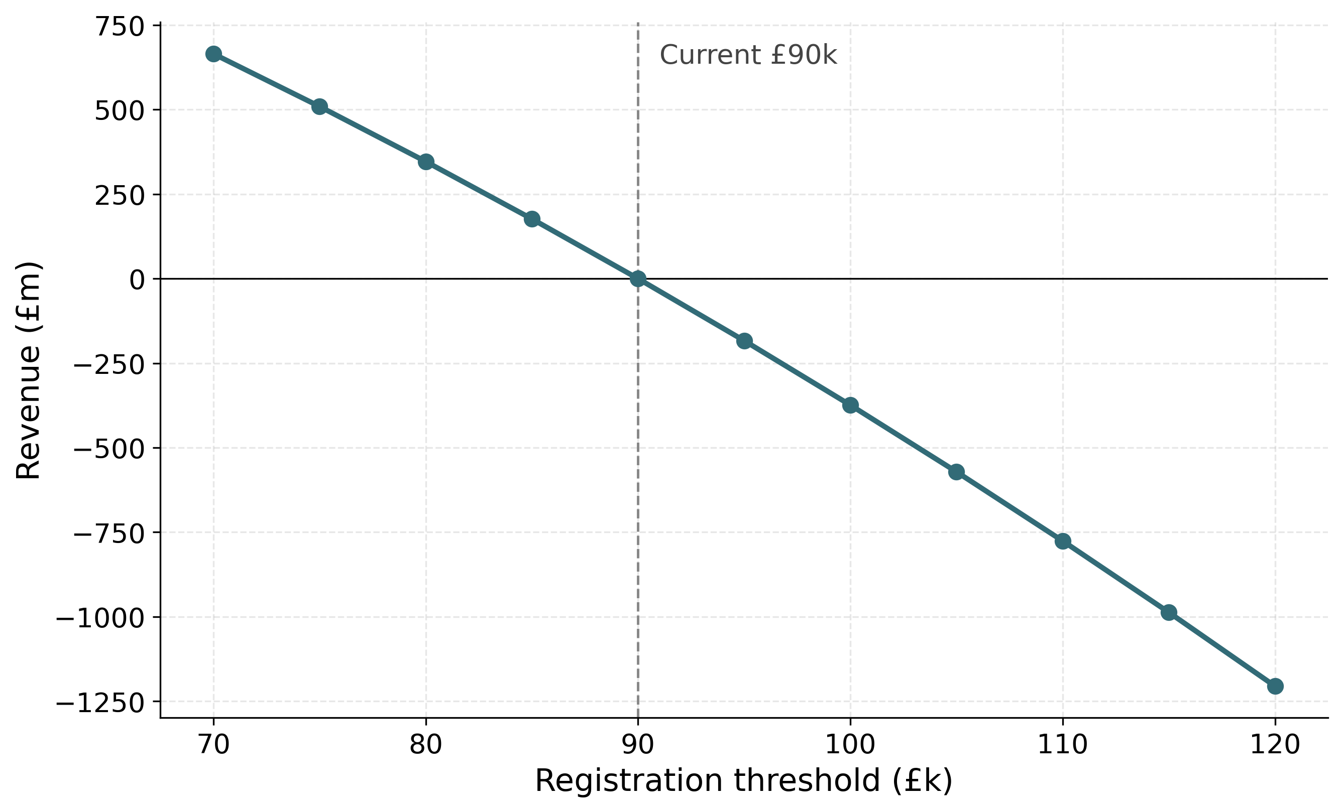
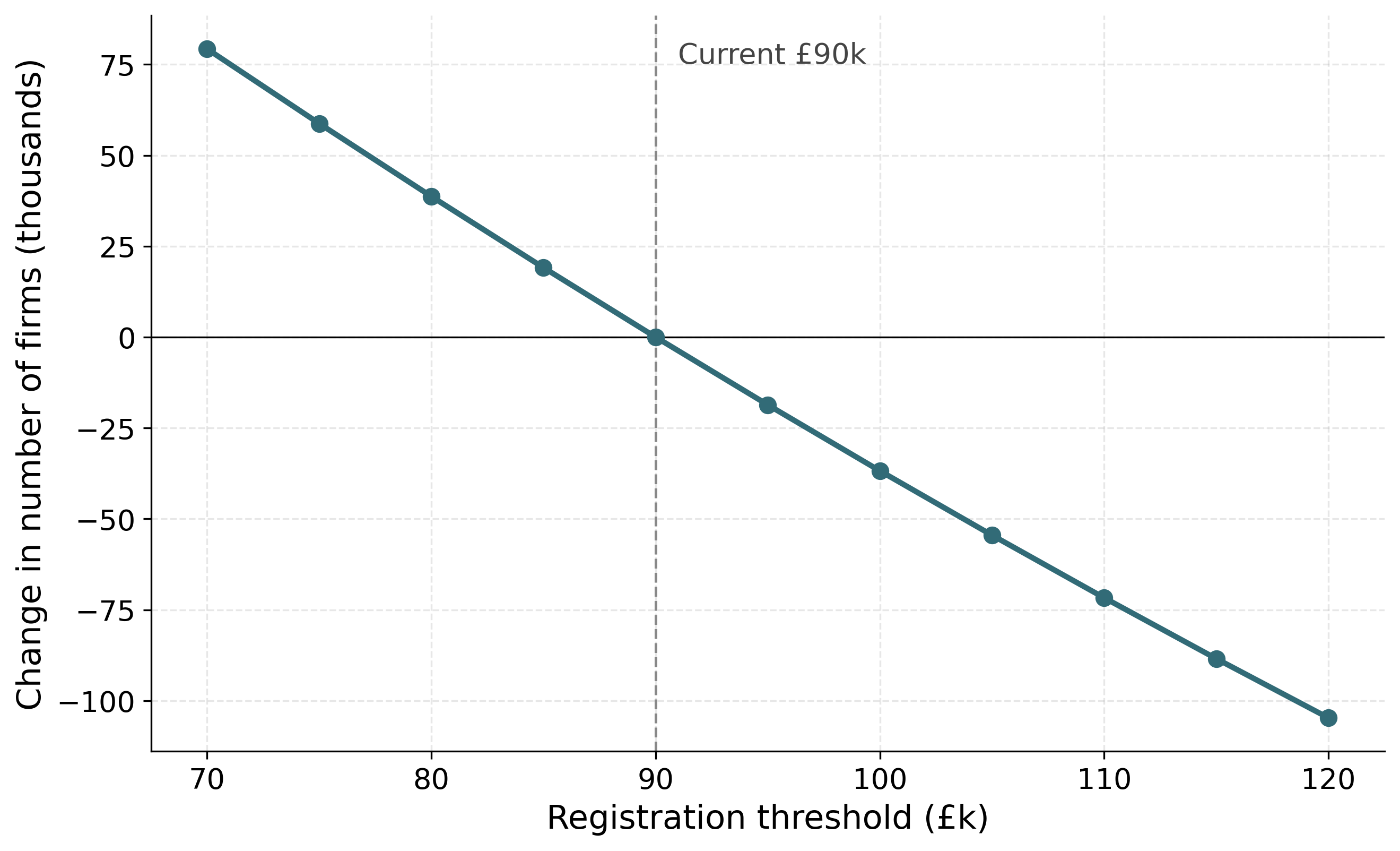
Having checked the method, I use it to cost a menu of further threshold locations, taking the post-reform £90,000 threshold as the baseline. Each row of Table 1 costs a move of the threshold to a new location for 2025–26, holding the turnover distribution fixed, so the revenue change reflects only the reclassification of firms into or out of the VAT net. Because the calibration places extra weight on high-liability firms just below the threshold, I evaluate the reclassified band from a smooth extrapolation of the clean above-threshold profile rather than the raw below-threshold mass. Lowering the threshold draws firms in and raises revenue; raising it loses revenue. The schedule is approximately linear, with a mild convexity as the threshold sweeps into denser parts of the distribution—each £5,000 step changes revenue by roughly £150m–£220m, with the marginal effect growing as the threshold sweeps across denser parts of the distribution. Even a £30,000 rise to £120,000 costs about £1.2bn, under \(0.6\%\) of the £203.8bn base, because the threshold governs many small firms whose individual liabilities are small. Figure 5 shows the sweep graphically. These are static results: they bound the first-order fiscal effect of a threshold change but abstract from the behavioural response of Section 5.
| Threshold | Revenue change (£m) | Change (%) | VAT-paying firms (000s) |
|---|---|---|---|
| £70,000 | \(+664.9\) | \(+0.33\) | \(+79.3\) |
| £75,000 | \(+509.0\) | \(+0.25\) | \(+58.7\) |
| £80,000 | \(+346.3\) | \(+0.17\) | \(+38.7\) |
| £85,000 | \(+176.6\) | \(+0.09\) | \(+19.1\) |
| £90,000 (baseline) | \(0\) | \(0\) | \(0\) |
| £95,000 | \(-183.5\) | \(-0.09\) | \(-18.6\) |
| £100,000 | \(-374.0\) | \(-0.18\) | \(-36.8\) |
| £105,000 | \(-571.4\) | \(-0.28\) | \(-54.5\) |
| £110,000 | \(-775.7\) | \(-0.38\) | \(-71.7\) |
| £115,000 | \(-987.0\) | \(-0.48\) | \(-88.5\) |
| £120,000 | \(-1{,}205.1\) | \(-0.59\) | \(-104.7\) |
Revenue impact (£m)
Change in VAT-paying firms (000s)
The threshold sweep above moves the location of a single cutoff. The same static method—re-applying a tax rule to the fixed turnover distribution, with no behavioural response—also costs reforms that change the shape of the schedule rather than merely its position. I consider four reforms and report their first-order revenue effects against a common baseline: the £85,000-notch / £183.6bn 2023–24 base. (This 2023–24 data-year base differs from the £203.8bn figure in the sweep above, which ages the same microdata to the 2025–26 fiscal year at the post-reform £90,000 threshold; the schedule reforms are costed in the data year to match the bunching and dominated-region analysis.) For each reform I recompute the weighted sum of liabilities \(R = \sum_i w_i\, v_i\) under the new schedule, holding each firm’s turnover fixed, and difference it against the baseline.
Raising the threshold from £85,000 to £100,000 is a pure location move, costed exactly as in the sweep above: it releases the firms with turnover in \([\pounds85{,}000, \pounds100{,}000)\)—about \(94{,}300\) firms—from the VAT net, for a static revenue change of \(-\)£508m on the £85,000-notch / £183.6bn base, consistent (same base) with the taper and reduced-rate reforms below. On this common base the level move is the most expensive option yet removes no distortion—it merely relocates the dominated region to a new cutoff—whereas the taper removes the dominated region entirely at lower cost (\(-\)£336m), foreshadowing Section 6.
A graduated taper replaces the discrete notch with an effective rate that phases linearly from \(0\%\) at £85,000 to the full \(20\%\) at £105,000. Firms in the band remit a tapered rather than a full rate on their (fixed) turnover; mechanically this reduces revenue by \(-\)£336m, with about \(123{,}100\) firms in the £85,000–£105,000 band facing a lower effective rate.
A banded reduced rate charges firms in the £85,000–£105,000 band a reduced rate \(\tau_{\text{low}}\in\{10\%,15\%\}\) in place of the standard \(20\%\), with \(20\%\) retained above £105,000. Statically this reduces revenue by \(-\)£343m at \(\tau_{\text{low}}=10\%\) and by \(-\)£171m at \(\tau_{\text{low}}=15\%\), again with about \(123{,}100\) firms in the band facing the lower rate.
| Reform | Lever | Static revenue (£m) |
|---|---|---|
| Raise threshold to £100,000 | Location | \(-508\) |
| Graduated taper \([\pounds85\text{k},\pounds105\text{k}]\) | Shape (phase-in) | \(-336\) |
| Reduced rate \(10\%\) \([\pounds85\text{k},\pounds105\text{k}]\) | Rate (step) | \(-343\) |
| Reduced rate \(15\%\) \([\pounds85\text{k},\pounds105\text{k}]\) | Rate (step) | \(-171\) |
These static figures bound the first-order fiscal effect of each reform but abstract from the behavioural response of Section 5. One feature of the shape reforms is not visible in a static costing: unlike a threshold move, which simply transports the notch to a new cutoff, the taper and the reduced rate change the size of the notch itself—the discrete drop in net revenue at the threshold and the empty band of turnover it induces. Quantifying that change requires the structural object I develop in Section 6, where I derive the notch’s dominated region and show analytically how each of these reforms alters it.
This section applies the polynomial counterfactual-density estimator of Saez (2010) and Kleven and Waseem (2013)—as used on UK VAT data by Liu et al. (2021)—to my synthetic firm population at the £85,000 registration threshold prevailing in my 2023–24 data. The estimator is purely reduced-form: it fits a smooth counterfactual to the empirical turnover density and reads excess mass off the gap, without imposing any structural model of the firm. My headline finding is one about my data rather than about firm behaviour. The estimator returns a sizeable excess-mass spike at the threshold, but a placebo test shows that this spike is mechanical: it is inherited from the coarse turnover-band targets I calibrate to, not generated by any location-choice in the synthetic firms. I therefore report the estimate as a reproduction of a published density step, stress-test it, and make no behavioural bunching claim and convert no excess mass into an elasticity. I read this as a transparency result: the open synthetic file faithfully transmits the administrative pattern, and its limit is reported openly.
Following Liu et al. (2021), I group firms into fine turnover bins of £100 and estimate a counterfactual density—the distribution that would obtain absent the registration notch—by polynomial regression on bin counts, excluding a manipulation window around the threshold \(y^{*}\): \[c_j \;=\; \sum_{l=0}^{q} \beta_l \, (y_j)^{l} \;+\; \sum_{i \in [y^{*}_{-},\, y^{*}_{+}]} \gamma_i \, \mathbb{1}\{j = i\} \;+\; \varepsilon_j ,\] where \(c_j\) is the number of firms in bin \(j\), \(y_j\) is the distance of bin \(j\) from the threshold, \(q\) is the polynomial order, and \([y^{*}_{-},\,y^{*}_{+}]\) is the excluded window. The fitted polynomial is then projected into the excluded region to recover the counterfactual density \(g(y)\). Excess bunching is the integrated difference between the observed and counterfactual densities just below the threshold, \[B(y^{*}) \;=\; \int_{y^{*}-\Delta y^{*}}^{y^{*}} g(y)\,\mathrm{d}y \;\approx\; g(y^{*})\,\Delta y^{*},\] the approximation holding when \(g\) is locally smooth. The bunching ratio \(b(y^{*}) = B(y^{*})/g(y^{*}) \approx \Delta y^{*}/y^{*}\) is the width of the bunching region expressed as a fraction of the threshold—a normalised ratio, not an elasticity. The estimator delivers the raw geometry of any density step at the threshold; whether that step reflects firm behaviour is a separate question, addressed by the placebo test below.
Applied to the 2023–24 synthetic data at the £85,000 threshold, the estimator returns a bunching ratio \(b = 0.060\) (SE \(0.005\)) and excess mass of \(8{,}712\) firms (SE \(662\)), with full inference—bootstrap standard errors and the mass-conservation restriction that excess mass below the threshold equal missing mass above it—reported in Appendix 9.2 and reproducible from the released code on the regenerated synthetic data. The observed density displays a clear step at the threshold: more mass in the £100 bins immediately below the cutoff than just above it.
I want to be precise about what this number is. It is the magnitude of a density step in my synthetic file, and that step reproduces the discontinuity documented in UK administrative micro-data by Liu et al. (2021): the open synthetic population transmits the published pattern. It is not a measured behavioural response. The synthetic generator contains no firm location-choice, so the firms in my file do not—and cannot—adjust their turnover to avoid registration. Whether the reproduced step nonetheless carries any behavioural information is exactly what the placebo test settles, and the answer is that it does not.
The central result of this section is a placebo test that diagnoses where the excess mass comes from. The test exploits a feature of my calibration targets. HMRC publishes turnover counts only in coarse bands across the threshold: \(678{,}350\) firms at or below £85,000 (an average of about \(7{,}981\) firms per £1,000) and \(305{,}320\) between £85,000 and £150,000 (about \(4{,}697\) per £1,000). The two band densities differ, so a step at £85,000 is already present in the calibration target before any firm is generated. Because the generator has no location-choice, any density discontinuity it produces must be inherited from this target rather than chosen by firms.
I therefore remove the step from the target in two ways and re-run the estimator. In Placebo A I reweight the existing synthetic firms so that the per-£1,000 density follows a single smooth trend across the threshold, holding total mass fixed. In Placebo B I replace the two HMRC band counts with a split implied by one common density, then regenerate the entire population and re-calibrate from scratch. The full table is in Appendix 9.2. The result is decisive: excess mass collapses from \(8{,}712\) firms to \(0\) under Placebo A and to \(99\) under Placebo B—about one per cent of the original spike—and the bunching ratio turns slightly negative in both. Removing the step from the calibration target removes essentially all of the bunching.
The conclusion I draw is plain. The synthetic bunching is inherited from the coarse HMRC band targets, not generated by firm behaviour, because the generator has no location-choice. I therefore make no behavioural bunching claim on these data, and I do not convert the excess mass into a turnover elasticity. The apparent agreement between my normalised statistic and LLAT’s (see below) is a mechanical coincidence fixed by the band-density ratio, not an independent behavioural match. This is a credibility result more than a negative one: the open synthetic file is stress-tested and its limit is reported transparently. The exercise also sits comfortably with the broader identification critique of bunching designs, which warns that excess mass need not point-identify a structural elasticity even in genuine administrative data (Blomquist et al. 2021; Bertanha et al. 2023); here the warning is sharper still, since the mass is not behavioural to begin with.
The behavioural fact in the literature is administrative. Liu et al. (2021) (hereafter LLAT) document genuine bunching at the same £85,000 UK VAT notch in HMRC micro-data, over a manipulation window of \(-\pounds14\)k to \(+\pounds24\)k, with an excess-bunching ratio of \(b = 1.361\) (SE \(0.202\)). If I normalise my synthetic excess mass to the same statistic I obtain \(b_{\mathrm{LLAT}} = 0.94\), of similar order of magnitude. I stress that this proximity is not an independent behavioural confirmation. As the placebo test above shows, my number is a mechanical reflection of the band-density ratio in the HMRC targets; its closeness to LLAT’s behavioural estimate is a coincidence of that ratio rather than a second measurement of the same response.
What does carry across is a piece of institutional context that both settings share. Like LLAT, the UK market features substantial voluntary registration below the threshold—LLAT report that almost half (roughly \(43\%\)) of eligible below-threshold firms register voluntarily—which dampens observed bunching relative to a pure turnover-tax notch and which my turnover-tax-notch model abstracts from. For wider order-of-magnitude context, Office for Budget Responsibility (2023) count firms holding turnover below the frozen threshold over a wide band (rising from \(23{,}000\) in 2017–18 to \(\sim 44{,}000\) in 2025–26, with foregone turnover of £110m rising to £350m); this is a different object from a near-threshold spike and is cited only as corroborating context, not as a like-for-like match.
The placebo sharpens, rather than weakens, the case for grounding the policy analysis in structure. The reduced-form density step cannot price reforms—it has no single point of excess mass to forward-map onto a change in the shape of the schedule—and on these data it cannot even be read behaviourally at all. What the structure of Section 6 does deliver exactly, for every reform considered, is the notch’s dominated region and how each schedule change alters it. It is precisely because the reduced-form bunching is non-identifying here that the exact dominated region carries the distortion characterisation. A fully behavioural forward solve that re-prices each firm’s turnover under counterfactual schedules would require further parameter-sensitive assumptions and is left to future work.
The behavioural response to the registration notch is documented in administrative data by Liu et al. (2021); on my synthetic data the reduced-form bunching is not behaviourally identified (Section 5). To characterise the notch precisely I therefore turn to its analytic structure, which yields an exact distortion measure that needs no behavioural calibration. I set out the firm-level structure following the framework of Kleven and Waseem (2013), Saez (2010), and Kleven (2016), as applied to UK VAT by Liu et al. (2021). The UK registration threshold is a notch, not a kink: once turnover crosses the threshold the firm becomes liable for VAT on its entire turnover, not merely on the increment above it. I model this notch exactly. The section’s central deliverable is the notch’s dominated region—an exact, model-free accounting identity that indexes the distortion the threshold imposes (Section 6.2), whose analytic response to each schedule reform complements the static reform costs of Section 4.1. The dominated region is a transparent, parameter-free distortion index: it depends on the rate and threshold alone and is therefore exact. Section 7 prices the behavioural response to each reform conditional on an assumed turnover elasticity, re-solving firm choices under each counterfactual schedule; here the dominated region remains the exact, elasticity-free distortion measure, requiring no assumption about the firm’s technology or elasticity.
The structure here taxes turnover. Real VAT is levied on value added with input-tax reclaim, and a substantial share of below-threshold firms register voluntarily to recover input VAT (Liu et al. 2021). My treatment abstracts from input reclaim and voluntary registration: it is a turnover-tax-notch approximation. This is a scope limitation I state up front; it bounds the welfare claims I make and is one I return to in the concluding discussion.
Each firm \(i\) chooses turnover \(y_i\) to maximise after-tax profit. Let \(c_i(y_i)\) denote the cost of producing turnover \(y_i\), \(T^{*}\) the registration threshold, and \(\tau\) the standard VAT rate. Because VAT applies to the firm’s entire turnover once it registers, after-tax revenue is discontinuous and profit is \[ \pi_i(y_i) \;=\; \begin{cases} \;y_i - c_i(y_i), & y_i < T^{*} \quad \text{(unregistered)},\\[4pt] \;(1-\tau)\,y_i - c_i(y_i), & y_i \ge T^{*} \quad \text{(registered)}. \end{cases} \tag{1}\] At \(T^{*}\) after-tax revenue falls discretely by \(\tau\,T^{*}\): a firm that nudges its turnover from just below to just above the threshold loses \(\tau\,T^{*}\) of net revenue on turnover it was already earning. With the standard rate \(\tau=0.20\) and threshold \(T^{*}=\pounds85{,}000\) this discrete drop is \(\tau\,T^{*}=\pounds17{,}000\). This drop—absent from a kink, where only the marginal rate changes at the threshold while average liability moves continuously—is the defining feature of a notch and the source of the bunching documented in Section 5. It is what makes locating just below the cutoff strictly attractive and creates the empty band derived in Section 6.2.
The notch creates a range of turnover just above \(T^{*}\) that no firm chooses, because every point in it yields strictly lower profit than locating at \(T^{*}\). A firm at the threshold earns net revenue \(T^{*}\); a registered firm at \(T^{*}+a\) earns \((1-\tau)(T^{*}+a)\). Equating the two—the cost difference across this narrow band is negligible—the upper edge of the dominated region is \[ (1-\tau)\,(T^{*}+a) \;=\; T^{*} \quad\Longrightarrow\quad a \;=\; T^{*}\,\frac{\tau}{1-\tau} . \tag{2}\] This is the Kleven–Waseem dominated-region width (Kleven and Waseem 2013). At my parameters it gives \(a = \pounds85{,}000\times 0.20/0.80 = \pounds21{,}250\), so the dominated region is \((T^{*},\,T^{*}+a)=(\pounds85{,}000,\ \pounds106{,}250)\), shown in Figure 7. Two properties make this \(\sim\pounds21\)k band a transparent, parameter-free index of the distortion. First, it is exact: it depends on \(\tau\) and \(T^{*}\) alone and is independent of the cost specification, of any behavioural elasticity, and of any smoothing parameter. Second, it is an order of magnitude wider than the \(\sim\pounds1\)k region implied by a smoothed kink approximation. The band also spans a populous part of the firm distribution: about \(137{,}000\) weighted firms in the synthetic population lie in the \(\pounds85{,}000\)–\(\pounds106{,}250\) dominated band, so the identity ranges over a heavily populated stretch of turnover rather than an empty tail. The \(15\%\) and \(10\%\) reduced-rate bands shrink the dominated zone to ranges containing about \(96{,}500\) and \(66{,}100\) firms respectively. The dominated region stands alone as a theoretical property of the schedule, independent of any reduced-form pattern in the data.
Because the width \(a=T^{*}\tau/(1-\tau)\) depends on the threshold and the rate alone, the effect of each schedule reform of Section 4.1 on this misallocation zone is exact and follows directly from Equation 2, with no dependence on the cost specification, any behavioural elasticity, or any simulated re-optimisation. Raising the threshold to £100,000 leaves the rate unchanged and therefore relocates the zone without altering its width: it is the same £21,250 band, transported to the new cutoff. A banded reduced rate shrinks the zone, because \(a\) falls with \(\tau\): at \(T^{*}=\pounds85{,}000\), lowering the band rate to \(15\%\) cuts it to \(\pounds85{,}000\times0.15/0.85=\pounds15{,}000\), and to \(10\%\) cuts it to \(\pounds85{,}000\times0.10/0.90=\pounds9{,}444\). A graduated taper has no notch and hence no dominated region: marginal net revenue declines smoothly through the band rather than off a cliff, so the band of dominated turnover—and with it the discrete incentive to suppress turnover—is removed entirely. The dominated region is thus the paper’s exact, model-free measure of the distortion the notch imposes, and the analytic statement above is exactly how much of that distortion each reform of Section 4.1 removes.
The reforms of Section 4 are costed statically: each schedule is re-applied to a fixed turnover distribution, and the revenue change is the mechanical reclassification of firms with no response in turnover. Section 5 then shows that the bunching in my synthetic data is mechanical, so a behavioural elasticity is not identified from it—the reduced-form response is a placebo. Section 6 supplies the one object that needs no behavioural calibration at all: the exact, model-free dominated region. What is missing from this sequence is the behavioural layer itself—a costing that lets firms re-optimise turnover when a reform changes the effective rate they face. This section supplies that layer. I build an iso-elastic structural simulator that, for an assumed turnover elasticity \(e\), re-solves each firm’s optimum under a counterfactual schedule and prices the resulting revenue effect. Because \(e\) is not identified from these data, I do not report a point estimate; I report an \(e\)-sensitivity range. The simulator nests the static costing of Section 4 as its \(e\to0\) limit, which I use below as a correctness check rather than treat as a coincidence. This is honest infrastructure, and every number in it is explicitly conditional on \(e\).
I adopt the iso-elastic firm problem of Kleven and Waseem (2013), in the sufficient-statistics tradition of Saez (2010) and as applied to UK VAT by Liu et al. (2021). A firm of ability \(n\) chooses turnover \(y\) to maximise \[ \pi(y;n) \;=\; \bigl(1-\tau(y)\bigr)\,y \;-\; \frac{n}{1+1/e}\left(\frac{y}{n}\right)^{1+1/e}, \tag{3}\] where \(\tau(y)\) is the effective VAT rate the schedule levies on the firm’s whole turnover once registered, and \(e>0\) is the elasticity of turnover with respect to the net-of-tax rate \(1-\tau\). Marginal cost is \((y/n)^{1/e}\), so the frictionless (\(\tau=0\)) optimum is \(y=n\): ability \(n\) is the firm’s undistorted turnover. A firm registered under a flat rate \(\tau\) chooses \[ y \;=\; n\,(1-\tau)^{e}, \tag{4}\] and one verifies directly from Equation 4 that \(\mathrm{d}\ln y / \mathrm{d}\ln(1-\tau) = e\), so \(e\) is exactly the knob that governs the intensive response.
To populate the simulator I recover an ability \(n\) for each firm from its observed turnover under the baseline £85,000 notch. Given \(e\), I set \(n=y_{\mathrm{obs}}\) for an unregistered firm (\(y_{\mathrm{obs}}<T^{*}\)) and invert Equation 4 for a registered firm, \(n=y_{\mathrm{obs}}/(1-\tau_i)^{e}\). The wedge \(\tau_i\) here is the firm’s own net VAT rate—net remittance over turnover, that is output VAT less input credits, which averages about \(3\%\) of turnover in the calibrated population (Section 3)—and not the statutory \(20\%\). This distinction is material: VAT is levied on value added, not on turnover, so a firm remitting \(3\%\) of its turnover has been distorted as if it faced a net-of-tax rate near \(0.97\), not \(0.80\). Inverting Equation 4 at the statutory \(20\%\) would inflate the recovered ability gap, and hence every counterfactual response, several-fold.
Holding the recovered abilities \(\{n_i\}\) and the assumed \(e\) fixed, I re-solve each firm’s optimum under the reform schedule—the raised threshold, the graduated taper, or the reduced-rate band—and aggregate the resulting liabilities. The behavioural revenue effect is the difference between this aggregate and the baseline. Because a reform that lowers the effective rate on the band raises each affected firm’s net-of-tax rate, the firm scales turnover up toward its frictionless optimum, \[ y^{*}_i \;=\; y_{\mathrm{obs},i}\, \left(\frac{1-\tau_{\mathrm{reform}}}{1-\tau_{\mathrm{base}}}\right)^{e} \;>\; y_{\mathrm{obs},i}, \tag{5}\] so the taxed base broadens and partly offsets the static loss.
I am explicit about what this exercise is and is not. Treating each firm’s observed (mechanically calibrated) turnover as optimal and inverting it for \(n\) is an accounting anchor, not structural identification: it reproduces the baseline by construction but borrows no information about the response. The elasticity \(e\) is not identified from these data (the placebo of Section 5), so every behavioural magnitude below is conditional on the assumed \(e\). The robust, \(e\)-free headline objects remain the static cost of Section 4 and the exact dominated region of Section 6; this section’s numbers are a disciplined sensitivity range, not point estimates. The margin priced here is purely intensive—firms scale turnover as the effective rate moves. The extensive notch distortion, the discrete incentive to suppress turnover and bunch below the threshold, is the separate analytic object of Section 6; a reader should not expect re-bunching dynamics here.
I sweep \(e\in\{0.05,\,0.17,\,0.32\}\) and take \(e=0.17\) as the headline. The low value \(0.05\) is of the order reported by Kleven and Waseem (2013); \(0.32\) is the mean implied by mapping the marginal-buncher condition through my notch; \(0.17\) is the median of that mapping. I flag the provenance plainly: the \(0.17\) and \(0.32\) values are read off the marginal-buncher condition applied to my notch geometry, which inherits the mechanical bunching that Section 5 shows to be non-behavioural, so they are model-implied, not data-identified; I use them only to delimit a plausible sweep, anchored at the lower end by the external Kleven and Waseem (2013) value, and a reader preferring a fully external range may substitute literature values for \(e\) directly without changing the conditional structure of the costing. The same mapping pins the marginal buncher \(n_H(e)\)—the highest ability that still finds it optimal to bunch at the threshold—at £112,795 for \(e=0.05\) (a frictionless excess of \(\Delta y^{*}\approx\pounds27.8\)k), £127,382 for \(e=0.17\) (\(\approx\pounds42.4\)k), and £143,527 for \(e=0.32\) (\(\approx\pounds58.5\)k), consistent with the analytic dominated-region width \(a=\pounds21{,}250\) of Section 6.
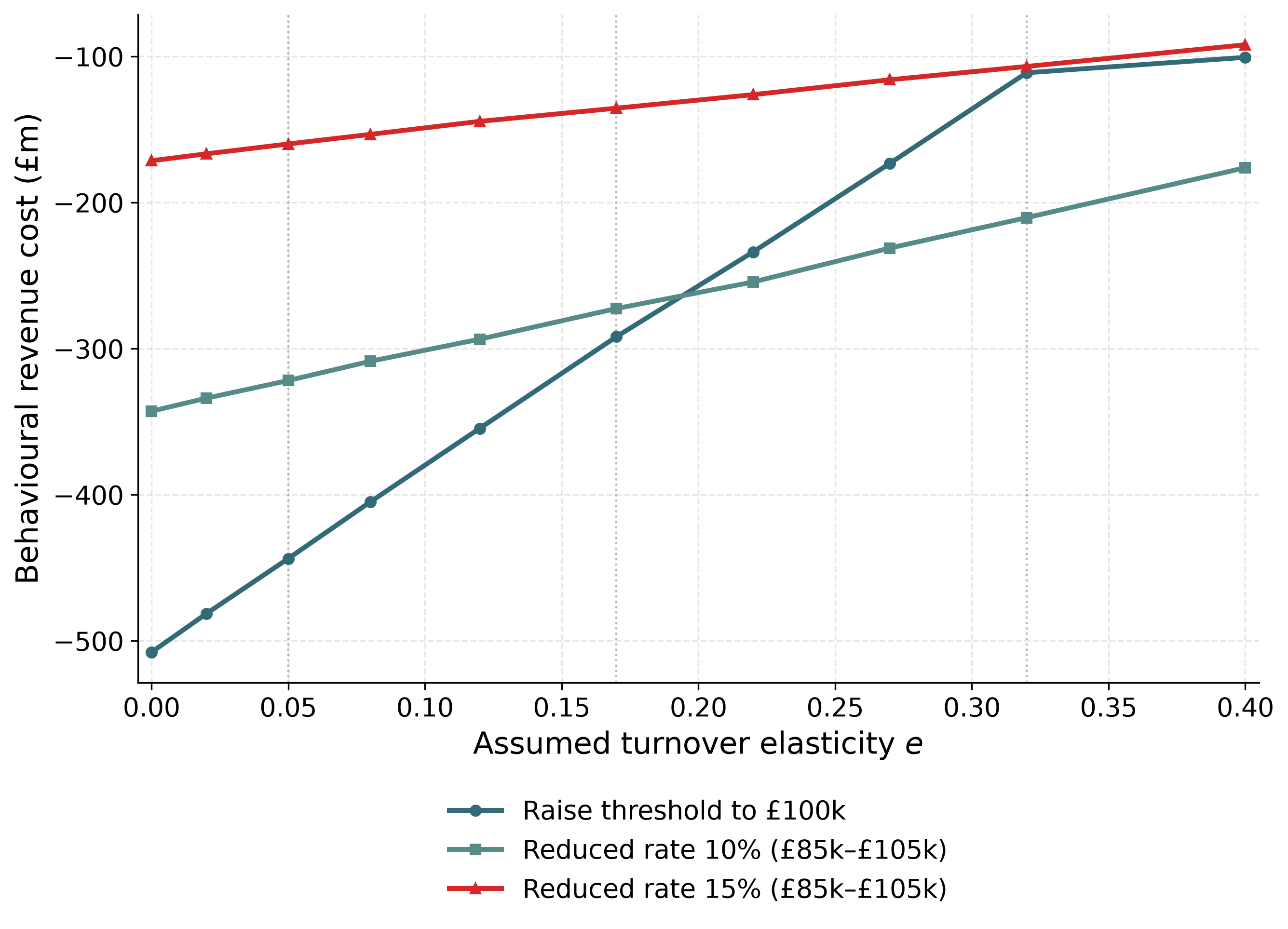
Table 3 reports the behavioural cost of each of the three flat-rate reforms—the raised threshold and the two reduced-rate bands—measured as the change in revenue relative to the £85,000-notch baseline, alongside the static figure of Table 2, for each \(e\). The direction is uniform across these three: a larger \(e\) makes each of them cheaper in revenue terms. The mechanism is Equation 5: each reform lowers the effective rate on the band by a constant amount, so firms scale turnover up toward their frictionless optimum, broadening the taxed base and partly offsetting the static loss. The offset is substantial: at \(e=0.17\) the raised threshold costs \(-\)£292m against a static \(-\)£508m, and the \(10\%\) and \(15\%\) bands cost \(-\)£273m and \(-\)£135m against static \(-\)£343m and \(-\)£171m. At the headline \(e=0.17\), the number of firms re-optimising is \(50{,}155\) under the raised threshold, \(61{,}187\) under the \(10\%\) reduced rate, and \(51{,}226\) under the \(15\%\) reduced rate. Figure 8 traces these costs across the full range of \(e\), with each curve nesting onto its static value as \(e\to0\).
I do not report a behavioural cost for the graduated taper, and I want to be candid about why. The taper carries two behavioural channels that pull in opposite directions. The first is the base-broadening channel shared with the flat reforms: as the average rate a firm faces falls, the firm scales its turnover up, which is cheaper for revenue in exactly the way Equation 5 captures. The second is a marginal-rate distortion that is the taper’s signature: because the taper’s rate rises with turnover, raising output lifts the rate on all of a firm’s turnover, so the firm faces an incentive to hold turnover down—a force that is costlier for revenue, not cheaper. The iso-elastic cost used here can price the first, upward channel but not the second, downward one. Imposing the full marginal-rate wedge in a correct first-order-condition solve makes firms collapse to the band floor and yields economically pathological revenue losses of the order of several billion pounds—an artefact of a cost function that cannot represent the downward, marginal-rate-driven response a taper induces, not a credible policy estimate. The net behavioural sign of the taper is therefore ambiguous and not identified in this framework. I take this as an honest scope limit, consistent with the paper’s careful identification stance, and report only the taper’s robust, \(e\)-free objects—its static cost (Section 4) and its exact, analytic removal of the dominated region (Section 6).
| Reform | Static | \(e=0.05\) | \(e=0.17\) | \(e=0.32\) | Firms (\(e{=}0.17\)) |
|---|---|---|---|---|---|
| Raise threshold to £100,000 | \(-\pounds508\)m | \(-\pounds444\)m | \(-\pounds292\)m | \(-\pounds111\)m | \(50{,}155\) |
| Reduced rate \(10\%\) \([\pounds85\text{k},\pounds105\text{k}]\) | \(-\pounds343\)m | \(-\pounds322\)m | \(-\pounds273\)m | \(-\pounds210\)m | \(61{,}187\) |
| Reduced rate \(15\%\) \([\pounds85\text{k},\pounds105\text{k}]\) | \(-\pounds171\)m | \(-\pounds160\)m | \(-\pounds135\)m | \(-\pounds107\)m | \(51{,}226\) |
Note. The graduated taper is deliberately omitted from this table. Its behavioural response cannot be credibly priced in the iso-elastic framework, for the reason set out in the paragraph below; its robust, \(e\)-free figures—the static cost of \(-\)£336m and the exact removal of the dominated region—are reported in Sections 4 and 6 instead.
For the three flat-rate reforms the simulator should reproduce the static costing as the response vanishes, and it does. Taking \(e\to0\) in the forward solve returns \(-\)£507m for the raised threshold, \(-\)£343m for the \(10\%\) reduced rate, and \(-\)£171m for the \(15\%\) reduced rate—matching the static \(-\)£508m, \(-\)£343m, and \(-\)£171m of Table 2 to within about £1m. This is the intended nesting: when no firm responds, the behavioural cost collapses to the mechanical reclassification effect, so the static costing is the \(e=0\) corner of the same machine, not a separate calculation. The nesting notably does not hold for the graduated taper—a further symptom that the iso-elastic cost cannot represent the taper’s marginal-rate channel, and an additional reason its behavioural cost is not reported. I separately confirm numerically that \(\mathrm{d}\ln y^{*}/\mathrm{d}\ln(1-\tau)=e\) holds exactly in the solved population for the flat reforms, so \(e\) is indeed the governing knob.
This section completes the costing framework. Where Section 4 prices each reform mechanically and Section 6 measures the distortion it removes, the simulator here prices the level and rate reforms behaviourally: it lets firms re-optimise turnover as the effective rate changes and implies that, for any assumed \(e\), the base-broadening response would offset a fraction of the static revenue loss. The layer is bounded by what it can and cannot identify. The behavioural magnitudes are conditional on an assumed, non-identified \(e\), and so are a sensitivity range rather than forecasts; and the priced margin is purely intensive, since the model re-scales turnover while holding the extensive bunching response fixed. Crucially, the graduated taper’s behavioural response is not credibly identified in this framework: its base-broadening and marginal-rate channels pull in opposite directions and the iso-elastic cost cannot net them, so I price it only statically and through its exact dominated-region removal. The robust anchors of the paper therefore remain the \(e\)-free static cost of Section 4 and the exact dominated region of Section 6; the contribution here is a disciplined, transparent layer that prices the intensive behavioural response to the level and rate reforms once one is willing to name an elasticity.
This paper contributes an open, reproducible firm-level microsimulation for analysing the UK VAT registration threshold, released in full—including its synthetic-data generator—for replication. Its value is as usable policy infrastructure rather than a structural identification result: I make no claim to recover policy-invariant firm primitives, unlike Garicano et al. (2016) and Gourio and Roys (2014). The analysis is anchored to the 2023–24 data year, in which the statutory threshold was £85,000. Table 4 collects the headline objects.
| Object | Symbol / definition | Value | Source |
|---|---|---|---|
| Static cost, £85k to £90k anchor | — | \(\approx-\pounds175\)m | §4 |
| Static sweep, £90k baseline | per £5k step | \(\sim\pounds150\)–\(220\)m | Table 1 |
| Dominated region (misallocation zone) | \(a=T^{*}\tau/(1-\tau)\) | £21,250 | §6.2 |
| Firms in the dominated band (weighted) | — | \(\approx137{,}000\) | §6.2 |
| Behavioural raise-to-£100k (\(e=0.05\)–\(0.32\)) | \(e\)-sensitivity range | \(-\pounds444\)m to \(-\pounds111\)m | §7 |
l-rate channels pull in opposite directions and the iso-elastic cost cannot net them, so only its static cost and dominated-region removal are reported. The static costs and the dominated region remain the robust, \(e\)-free anchors; the behavioural magnitudes are conditional on the assumed \(e\).
The model is a turnover-tax-notch approximation: it treats VAT as a cost on turnover, whereas real VAT is levied on value added with input reclaim, and roughly half of below-threshold firms register voluntarily (Liu et al. 2021), so the effective notch is smaller than a flat treatment implies. The microdata are synthetic and calibrated to coarse aggregate bands—which is why the behavioural magnitudes are reported only conditional on an assumed elasticity rather than as estimates—and the analysis is partial-equilibrium, abstracting from pass-through into prices (Benedek et al. 2015; Bellon et al. 2022). The conditional behavioural costing is now done (Section 7), but on synthetic data the turnover elasticity \(e\) it requires is assumed, not identified; the chief outstanding task is therefore to identify \(e\) from administrative micro-data, which would turn the present \(e\)-sensitivity range into a point estimate. A welfare/MVPF analysis modelling value added and input reclaim would in turn convert the dominated-region distortion into cost–benefit terms and support revenue-neutral schedule designs that neutralise the notch at no net fiscal cost. Above all, validation against administrative firm-level data with genuine location choice would replace the present internal-consistency checks with out-of-sample tests and let the framework identify firm bunching directly.
This appendix collects supporting material in two parts: data construction and calibration robustness (Appendix 9.1); and statistical inference for the reduced-form bunching estimates (Appendix 9.2), which also reports a placebo test demonstrating that the synthetic bunching is mechanical—inherited from the coarse HMRC turnover-band targets—rather than behavioural.
Section 3 describes the two-stage synthetic-population pipeline, parameterised by the registration threshold, and its calibration to HMRC and ONS aggregates. This appendix records the implementation detail deferred from that account.
Each of the approximately \(2.94\) million firm rows carries a turnover, an input expenditure, a calibration weight, and a registration status; the weights are chosen so the weighted totals reproduce the official targets while the population sums to about \(2.5\) million firms. Because the population is calibrated to the HMRC aggregates, agreement between my weighted outputs and those aggregates is a check of internal consistency, not external validation: any target used in calibration is reproduced by construction. I therefore read the \(\sim\!90\%\) calibration accuracy, and the close match of the static £85,000 \(\to\) £90,000 costing to HMRC’s published figures, as consistency checks on the pipeline rather than out-of-sample tests of firm behaviour.
The reported calibration score is a bounded summary statistic. For each dimension I compute \(\max\{0,1-\lvert \widehat{T}-T\rvert/\lvert T\rvert\}\), so a dimension missed by more than 100 percent receives zero rather than a negative score. The headline “overall” number is the unweighted mean of the five dimensions used as calibration targets—HMRC turnover bands, ONS population, employment bands, HMRC sector counts, and VAT liability by turnover band. VAT liability by sector is excluded from that mean and reported separately as an informational diagnostic, because the current generator does not calibrate sector-specific input/output VAT structure.
The no-VAT counterfactual density of Section 5 is fitted by polynomial regression on the observed density outside a manipulation window around the threshold. The baseline excludes \([T^{*}-15\text{k}, T^{*}+15\text{k}]\) and fits a cubic. Widening the window guards against contamination of the counterfactual by the behavioural response but reduces the data available for the fit; raising the degree improves in-sample fit but risks over-fitting the tails. The sensitivity of the excess-mass and bunching-ratio estimates to window width and degree, with associated uncertainty, is reported in Appendix 9.2.
This appendix documents the inference procedure for the reduced-form bunching estimates of Section 5: the mass-conservation constraint that disciplines the counterfactual density, the bootstrap that delivers standard errors, the sensitivity of the estimates to the polynomial degree, the exclusion window, and the effective wedge \(\tau_{e}\), and a placebo test demonstrating that the synthetic bunching is mechanical rather than behavioural. All numbers reported here and in the calibration step are produced by the released estimator (fixed seed, \(B=200\) bootstrap replications), run on the £85,000 (2023–24) weighted synthetic firm data; the seed and \(B\) are fixed so the table is reproducible, and nothing is hardcoded as a result.
The canonical bunching estimator of Saez (2010), Kleven and Waseem (2013) and Chetty et al. (2011) imposes that the counterfactual density conserves mass: every firm removed from above the threshold reappears as excess mass below it. An unconstrained fit by plain polynomial OLS on bins outside a hand-set window computes the excess mass \(E\) (below \(T^{*}\)) and the missing mass \(\Delta_{R}\) (above \(T^{*}\)) independently, with no guarantee that \(E = \Delta_{R}\) and no endogenous location of the marginal buncher.
I impose the constraint in two ways. First, the counterfactual polynomial in \((y-T^{*})\) is fit by an iterated weighted least-squares procedure in which the density of the bins above the excluded region is rescaled until the fitted counterfactual integrates to the observed total mass over the estimation range \([\pounds20\text{k},\pounds140\text{k}]\). This forces the bunching mass to be reabsorbed into the counterfactual rather than discarded. The regressor is normalised to \([-1,1]\) for numerical stability of the high-degree Vandermonde basis. Second, the upper edge of the excluded (manipulation) region—the marginal buncher \(y_{R}\)—is located endogenously by integrating the missing mass upward from \(T^{*}\) until cumulative missing mass above equals cumulative excess mass below, \[\int_{T^{*}}^{y_{R}} \bigl[f^{\mathrm{cf}}(y)-f^{\mathrm{obs}}(y)\bigr]_{+}\,dy \;=\; \int_{T^{*}-W}^{T^{*}} \bigl[f^{\mathrm{obs}}(y)-f^{\mathrm{cf}}(y)\bigr]_{+}\,dy \;=\; E ,\] rather than being fixed at an arbitrary window edge. The excess turnover span of the marginal buncher, \(\Delta y^{*}=y_{R}-T^{*}\), is then used by the notch-width elasticity.
Imposing the constraint matters because the unconstrained fit grossly violates adding-up: it delivers \(E=7{,}820\) but \(\Delta_{R}=16{,}524\), whereas the constrained estimator returns \(E=8{,}712\) and \(\Delta_{R}=9{,}214\), which agree to within sampling noise. Imposing the constraint thus reconciles the excess mass below the threshold with the missing mass above it, which the unconstrained estimator computes independently and which would otherwise diverge by roughly a factor of two; the resulting movement in the headline estimates is reported in the calibration step.
I compute standard errors by a firm-level bootstrap. In each of \(B=200\) replications I draw \(n\) firms with replacement from the estimation sample, with draw probabilities proportional to the survey weight, re-bin the resampled firms into £1,000 bins, and re-run the entire estimator—counterfactual fit, marginal-buncher location, and all downstream statistics—on the replicate. The standard error of each statistic is the standard deviation of its bootstrap distribution, and the \(95\%\) confidence interval is the \(2.5\)th–\(97.5\)th percentile interval. Resampling firms (rather than residuals) propagates both sampling variation and the variation induced by re-binning. Table 5 reports the results.
| Statistic | Point | Std. error | 95% CI |
|---|---|---|---|
| Bunching ratio \(b\) | \(0.060\) | \(0.005\) | \([0.050,\ 0.068]\) |
| Excess mass \(E\) | \(8{,}712\) | \(662\) | \([7{,}920,\ 10{,}516]\) |
| Substitution elasticity \(\sigma\) | \(4.85\) | \(0.12\) | \([4.58,\ 5.08]\) |
| Displaced share \(\Pi\) | \(0.211\) | \(0.005\) | \([0.200,\ 0.219]\) |
| Notch-width elasticity (median) | \(0.448\) | \(0.027\) | \([0.405,\ 0.496]\) |
| Marginal-buncher elasticity | \(0.657\) | \(0.082\) | \([0.510,\ 0.821]\) |
The bunching-implied elasticities in Table 5—the notch-width elasticity (\(\approx 0.45\)) and the marginal-buncher elasticity (\(\approx 0.66\))—together with the CES substitution elasticity \(\sigma = 4.85\) are not behaviourally identified on these data. The synthetic firm population is calibrated to coarse aggregate HMRC turnover-band counts, and the generator contains no firm location-choice: firms do not respond to the threshold, so the excess mass below it is mechanical, inherited from the density step in the calibration targets rather than from any behavioural response (the placebo test below makes this precise). The elasticities are therefore reported only as a record of what the estimator returns when applied to these data; the paper draws no behavioural conclusion from them. This is an instance of the general non-identification of bunching elasticities absent exogenous variation or strong functional-form assumptions (Blomquist et al. 2021; Bertanha et al. 2023).
Table 6 maps the point estimates across a grid of polynomial degree \(\in\{5,6,7,8\}\) and symmetric exclusion window \(\in\{\pounds10\text{k},\pounds15\text{k},\pounds20\text{k},\pounds25\text{k}\}\). The estimates are stable across the central cells (degree \(6\)–\(7\), window £10–£20k): the substitution elasticity stays in roughly \(4.4\)–\(5.7\) and the excess mass in \(4{,}000\)–\(9{,}000\). The corner cells are less reliable: at very wide windows (\(\pounds25\)k) the excluded region begins to swallow genuine curvature in the density, the fitted counterfactual crosses the observed density, and \(b\) can turn slightly negative (so \(\sigma\) is undefined); at the lowest degree (\(5\)) the inflexible trend over-fits the bunching mass into the counterfactual and inflates \(b\). I therefore report the degree-\(7\), £15k-window specification as the baseline, with the bootstrap CIs above spanning the variation across the stable interior of the grid.
| Degree | Window | \(b\) | \(E\) | \(\sigma\) | Notch-width (median) |
|---|---|---|---|---|---|
| 6 | £10k | \(0.077\) | \(7{,}262\) | \(5.42\) | \(0.41\) |
| 6 | £15k | \(0.045\) | \(6{,}575\) | \(4.99\) | \(0.44\) |
| 6 | £20k | \(0.015\) | \(3{,}822\) | \(4.21\) | \(0.35\) |
| 7 | £10k | \(0.091\) | \(8{,}539\) | \(5.07\) | \(0.47\) |
| 7 | £15k | \(\mathbf{0.060}\) | \(\mathbf{8{,}712}\) | \(\mathbf{4.85}\) | \(\mathbf{0.45}\) |
| 7 | £20k | \(0.034\) | \(7{,}313\) | \(4.62\) | \(0.43\) |
The CES substitution elasticity is recovered as \(\sigma = \ln(\mathrm{RR})/\ln(1+\tau_{e})\), where \(\mathrm{RR}\) is the ratio of counterfactual-to-observed above/below mass ratios. Because the wedge enters only through \(\ln(1+\tau_{e})\), \(\sigma\) scales roughly as \(1/\ln(1+\tau_{e})\) while the displaced share \(\Pi = 1-(1+\tau_{e})^{-\sigma}\) is essentially invariant (it is pinned by \(\mathrm{RR}\)). On my data, \(\tau_{e}=0.025\) gives \(\sigma=9.59\), \(\tau_{e}=0.05\) gives \(\sigma=4.85\), \(\tau_{e}=0.075\) gives \(\sigma=3.28\), and \(\tau_{e}=0.10\) gives \(\sigma=2.49\), while \(\Pi=0.211\) throughout. The magnitude of \(\sigma\) is therefore conditional on \(\tau_{e}\): I adopt \(\tau_{e}=0.05\) as a baseline effective registration wedge and report \(\Pi\), which is robust to it, as the policy-relevant displacement object.
The non-identification of the bunching elasticities can be made precise with a placebo test. The HMRC turnover-band targets to which the synthetic population is calibrated are coarse: a single count for firms at or below £85,000 and a single count for firms in £85,000–£150,000. The implied average per-£1,000 densities differ sharply across the threshold (\(\approx 7{,}981\) firms/£1,000 below versus \(\approx 4{,}697\) above), so the calibration target itself contains a density step at exactly £85,000. Because the generator has no firm location-choice, any density discontinuity in the synthetic population must be inherited from this stepped target rather than produced by behaviour. The placebo removes the step and re-runs the estimator. Table 7 reports two variants: Placebo A reweights the existing synthetic firms so the per-£1,000 density follows a single smooth log-quadratic trend across the threshold (preserving total mass over \([\pounds20\text{k},\pounds140\text{k}]\), no regeneration); Placebo B replaces the two HMRC band counts straddling £85,000 with a split implied by a single common per-£1,000 density (no step in the target), then re-runs the full generator and multi-objective calibration before estimating.
| Population | \(b\) | \(E\) | \(b_{\mathrm{LLAT}}\) |
|---|---|---|---|
| Actual (control) | \(+0.060\) | \(8{,}712\) | \(0.941\) |
| Placebo A (reweight density smooth) | \(-0.063\) | \(0\) | \(0.000\) |
| Placebo B (un-stepped HMRC band targets) | \(-0.016\) | \(99\) | \(0.010\) |
When the density step is removed from the calibration target, the estimated excess mass collapses from \(8{,}712\) firms in the control to at most \(\approx 99\) firms (\(\approx 1\%\) of the control value) in Placebo B, and to zero in Placebo A; the bunching ratio even turns slightly negative. This proves that the synthetic bunching is inherited from the coarse HMRC turnover-band targets, not from any firm behaviour, and confirms that the elasticities in Table 5 are mechanical artefacts of the calibration rather than behavioural parameters. The placebo is part of the released code and is fully reproducible.